Google Sheets VLOOKUP Function
VLOOKUP Function
The VLOOKUP function is a premade function in Google Sheets, which allows searches across columns.
It is typed =VLOOKUP and has the following parts:
=VLOOKUP(search_key, range,
index, [is_sorted])
Note: The column which holds the data used to lookup must always be to the left.
serach_key: Select the cell where search values will be entered.
range: The table range, including all cells in the table.
index: The data which is being looked up. The input is the number of the column, counted from the left:
[is_sorted]: TRUE/1 if the range is sorted or FALSE/0 if it is not sorted.
Note: Both 1 / 0 and True / False can be used in [is_sorted].
Let's have a look at an example!
Vlookup Function Example
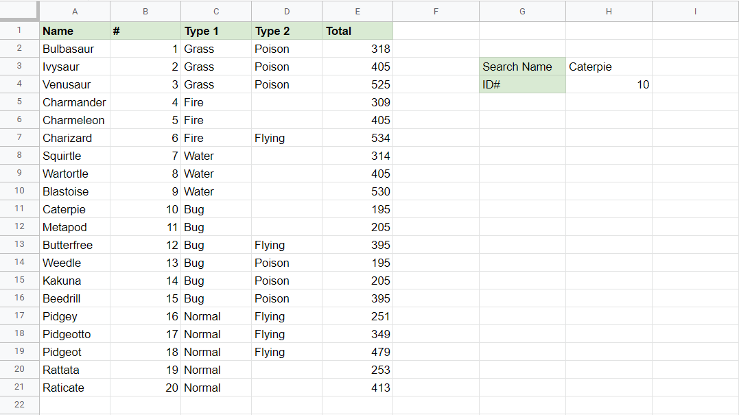
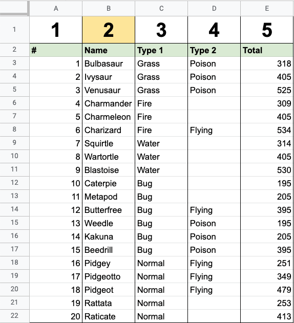
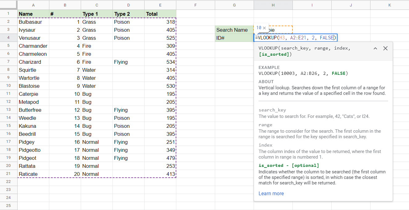
Lookup and return Pokemon names from this list by their ID#:
The VLOOKUP function, step by step:
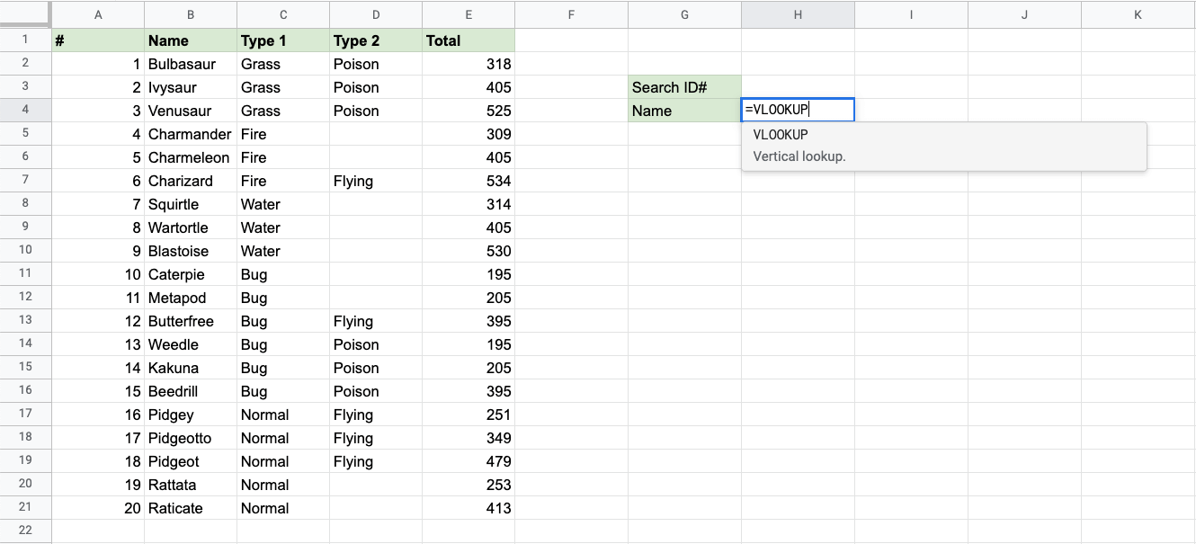
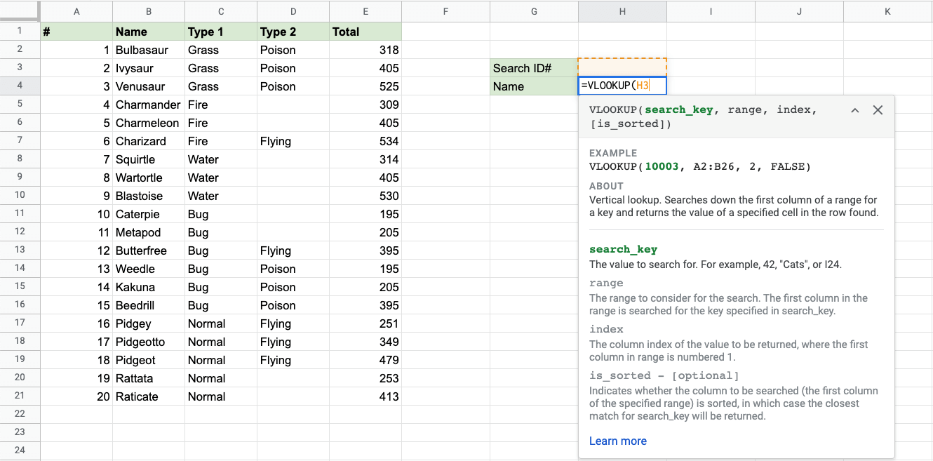
- Select the cell
H4 - Type
=VLOOKUP - Click the VLOOKUP command
H4 is where the search result is displayed. In this case, the Pokemon's names based on their ID#.
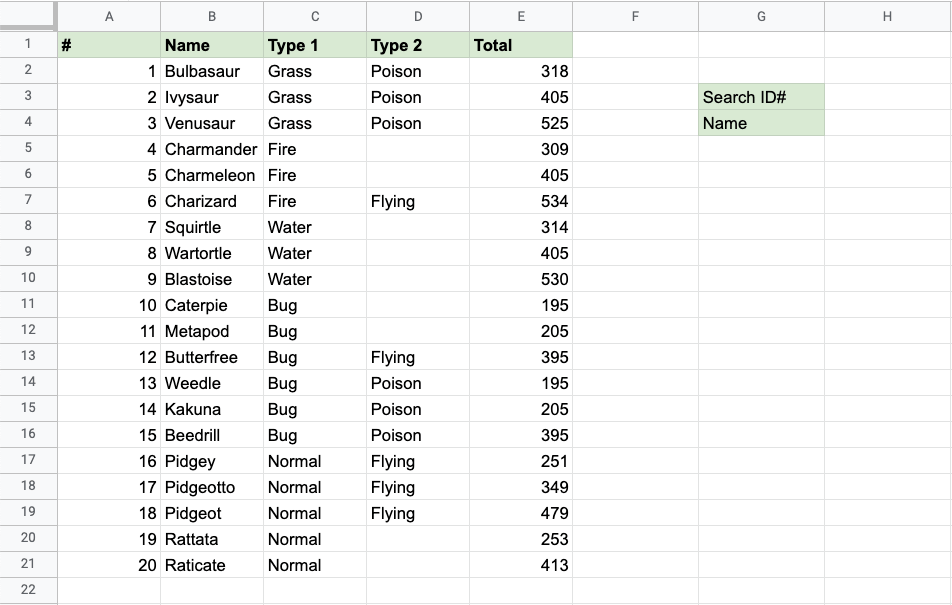
- Select the cell where search value will be entered (
H3)
H3 selected as serach_key. This is the cell where the search query is entered. In this case the Pokemon's ID#.
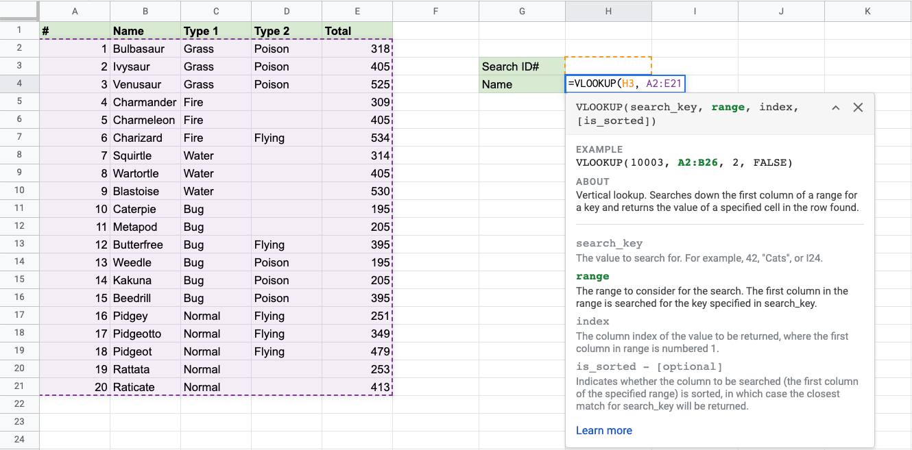
- Type
, - Specify the table range
A2:E21
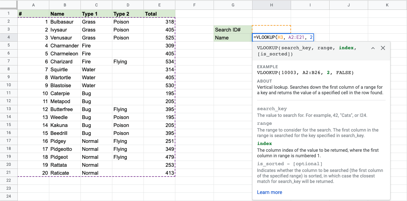
- Type
, - Type the number of the Name column, counted from the left:
2
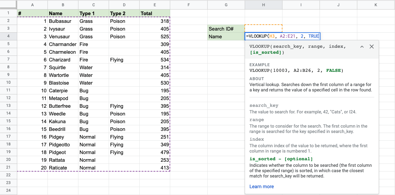
- Type
TRUE - Hit enter
In this example the table is sorted by ID#, so the [is_sorted] value is TRUE.
An illustration for selecting column index number 2:
Now, the function returns the Name value of the search_key specified in cell H3:

Good job! The function returns the #N/A value. This is because there have not been entered any value to the Search ID# cell H3.
Let us feed a value to it, type 7 into cell H3:
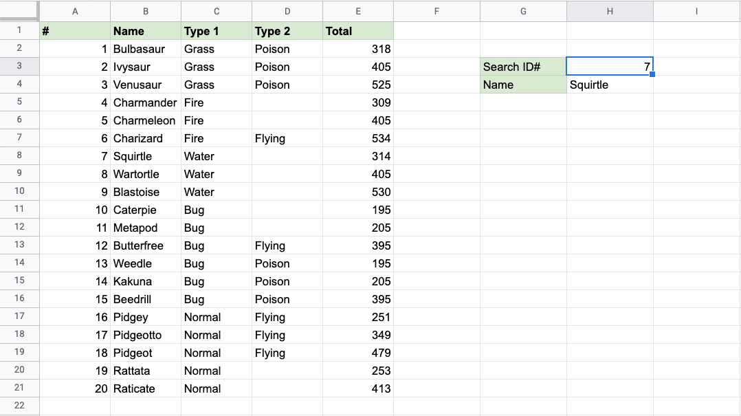
Have a look at that! The VLOOKUP function has successfully found the Pokemon Squirtle which has the ID# 7.
One more time, type 4 into cell H3:
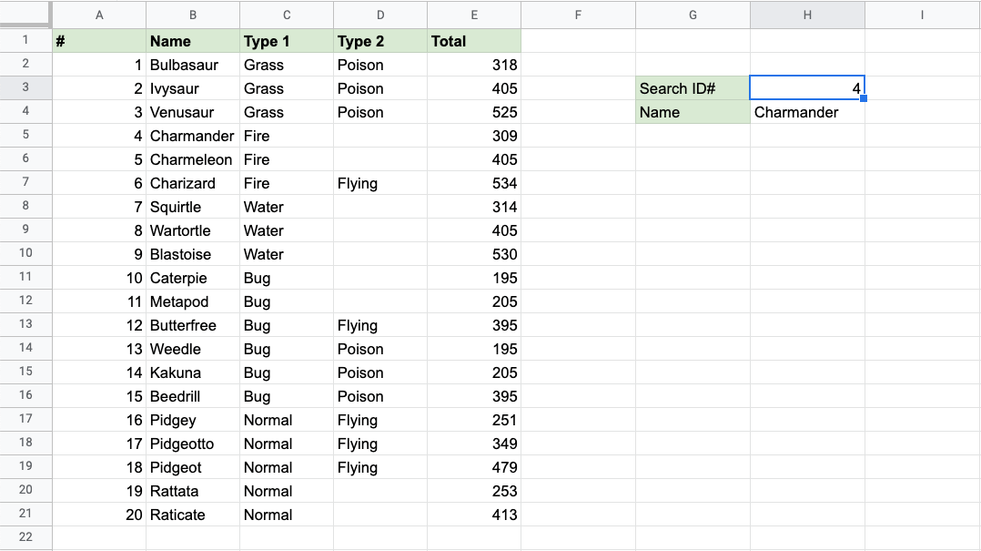
It still works! The function returned Charmanders name, which has 4 as its ID#. That's great.
Let's try another example, using the Pokemon names as input instead.
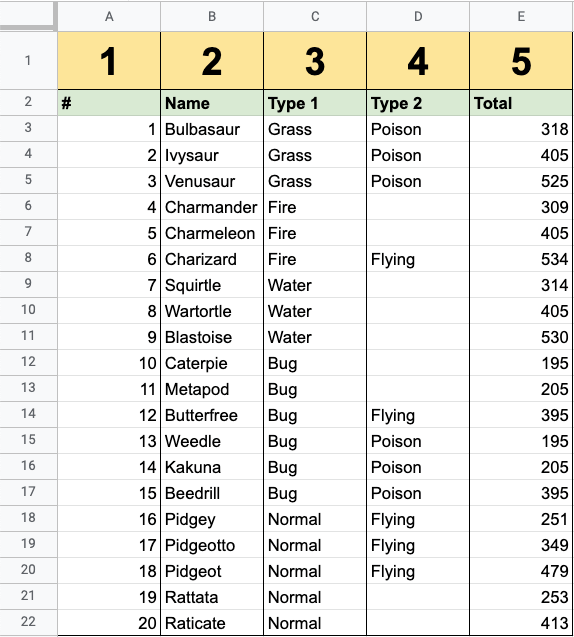
First, change the places of columns A and B.
Note: You can click and drag coloumns in Google Sheet to rearrange them.
Clicking and holding coloumn A and dragging it between columns B and C will rearrange them like this:
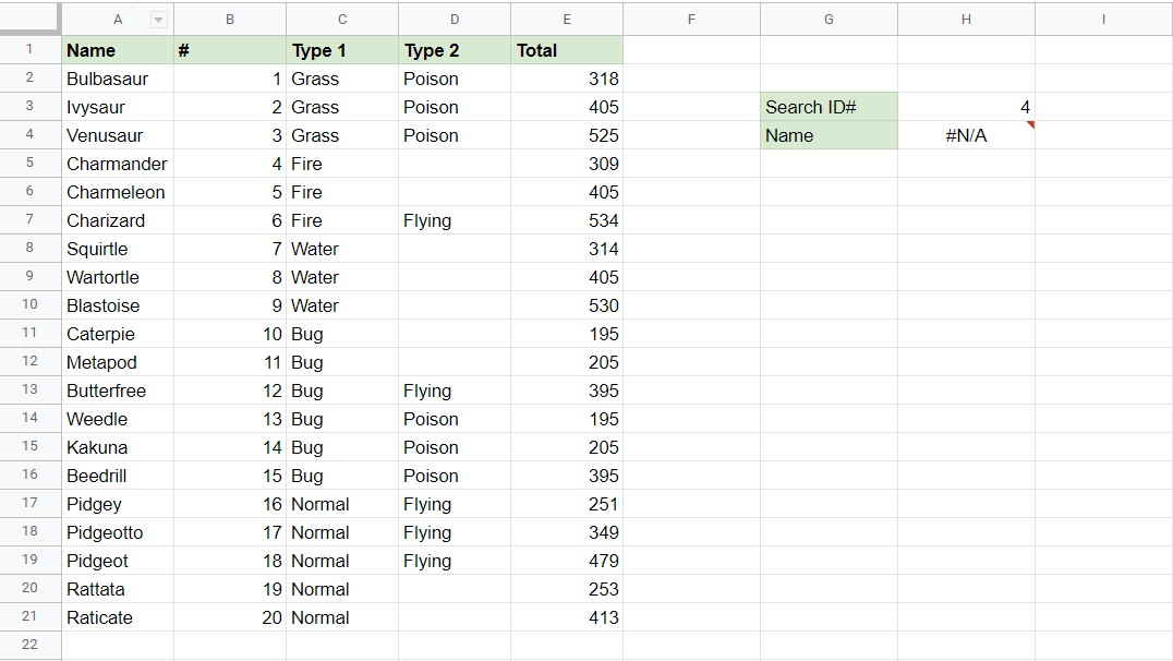
Now, the function is trying to look up 4 in the Name column, which returns the #N/A error.
Let's switch the labels, and try to enter Caterpie into the cell H3, where the vlookup functions finds the search_key:

Notice that the ID# returned is 1, although Caterpie's ID# is actually 10.
This result is another error.
This is because the Name values are not sorted like the ID numbers are.
Let's change the value of the [is_sorted] part of the function from TRUE to FALSE:
Now, the function correctly returns Caterpie's real ID number: